Librerías requeridas: dplyr, flextable6 Replicación en R de caso de estudio: Hayashi (2014)
Cápitulo 3: Latent structure analysis of the process variables and pharmaceutical responses of an orally disintegrating tablet
7 Artículo de estudio
El artículo de Hayashi (2014) tiene como objetivo la optimización y el análisis del proceso de fabricación de tabletas orodispersables (ODTs) de indometacina dentro del marco de Calidad por Diseño (QbD).
En este estudio se emplea un diseño Box–Behnken, considerando como factores experimentales la cantidad de agua (AGUA), Tiempo de amasado (T_AMA), fuerza de compresión(F_COMP) y cantidad de estearato de magnesio (EST_MG) (véase la Tabla 16.1).
Las matrices del diseño, tanto en unidades codificadas como en unidades naturales, se presentan en la Tabla 16.2. Las variables respuesta analizadas son la fuerza tensil (TS) y el tiempo de desintegración (TD).
A continuación, se muestra la réplica del experimento reportado por Hayashi (2014) para la respuesta fuerza tensil (TS).
Variables | Nivel (-1) | Nivel (0) | Nivel (1) |
|---|---|---|---|
Cantidad de agua (AGUA) | 30% | 35% | 40% |
Tiempo de amasado (T_AMA) | 1 min | 5 min | 9 min |
Fuerza de compresión (F_COMP) | 3 kgf | 4 kgf | 5 kgf |
Cantidad de Est.magnesio (EST_MG) | 0.5% | 1.5% | 2.5% |
Nota
Véase “Guía para la implementación de diseños experimentales en la industria farmacéutica” para una explicación detallada de los cálculos presentados.
8 Simulación de respuestas
El artículo de Hayashi (2014) reporta únicamente el valor promedio de las tres réplicas junto con su desviación estándar, por lo que se requiere simular los datos individuales. Para este propósito, se construyó la función simuesblo, disponible en el archivo funciones.R del repositorio ncortes/Disexp_Industria_Farmaceutica en GitHub (funcionesR?).
Código
# Variables respuesta
TS_media = c(0.85, 1.12, 1.00, 1.28, 0.74, 0.81, 1.42, 1.51, 0.99, 1.10, 1.20, 1.33, 0.68, 1.17, 0.74, 1.47, 0.75, 1.36, 0.94, 1.65, 0.79, 0.91, 1.08, 1.17, 1.16, 1.17, 1.13)
TS_sd    = c(0.01, 0.03, 0.08, 0.04, 0.01, 0.02, 0.03, 0.08, 0.04, 0.05, 0.07, 0.06, 0.01, 0.06, 0.03, 0.09, 0.01, 0.05, 0.01, 0.06, 0.05, 0.03, 0.02, 0.02, 0.05, 0.05, 0.02)

TS <- as.vector(simuesblo(TS_media, TS_sd, 3, 2))
9 Construcción de diseño Box–Behnken
A continuación se presenta la réplica del artículo presentado por Hayashi (2014)
Código
# Diseño
des <- data.frame(
  x1 = rep(c(-1, -1,  1,  1,  0,  0,  0,  0, -1, -1,  1,  1,  0,  0,  0,  0, -1, -1,  1,  1,  0,  0,  0,  0, 0, 0, 0),3),
  x2 = rep(c(-1,  1, -1,  1,  0,  0,  0,  0,  0,  0,  0,  0, -1, -1,  1,  1,  0,  0,  0,  0, -1, -1,  1,  1, 0, 0, 0),3),
  x3 = rep(c( 0,  0,  0,  0, -1, -1,  1,  1,  0,  0,  0,  0, -1,  1, -1,  1, -1,  1, -1,  1,  0,  0,  0,  0, 0, 0, 0),3),
  x4 = rep(c( 0,  0,  0,  0, -1,  1, -1,  1, -1,  1, -1,  1,  0,  0,  0,  0,  0,  0,  0,  0, -1,  1, -1,  1, 0, 0, 0),3),
  TS)
TRAT | AGUA(c) | T_AMA(c) | F_COMP(c) | EST_MG(c) | AGUA(n) | T_AMA(n) | F_COMP(n) | EST_MG(n) | TS |
|---|---|---|---|---|---|---|---|---|---|
1 | -1 | -1 | 0 | 0 | 30 | 1 | 4 | 1.5 | 0.85 |
2 | -1 | 1 | 0 | 0 | 30 | 9 | 4 | 1.5 | 1.12 |
3 | 1 | -1 | 0 | 0 | 40 | 1 | 4 | 1.5 | 1.00 |
4 | 1 | 1 | 0 | 0 | 40 | 9 | 4 | 1.5 | 1.28 |
5 | 0 | 0 | -1 | -1 | 35 | 5 | 3 | 0.5 | 0.74 |
6 | 0 | 0 | -1 | 1 | 35 | 5 | 3 | 2.5 | 0.81 |
7 | 0 | 0 | 1 | -1 | 35 | 5 | 5 | 0.5 | 1.42 |
8 | 0 | 0 | 1 | 1 | 35 | 5 | 5 | 2.5 | 1.51 |
9 | -1 | 0 | 0 | -1 | 30 | 5 | 4 | 0.5 | 0.99 |
10 | -1 | 0 | 0 | 1 | 30 | 5 | 4 | 2.5 | 1.10 |
11 | 1 | 0 | 0 | -1 | 40 | 5 | 4 | 0.5 | 1.20 |
12 | 1 | 0 | 0 | 1 | 40 | 5 | 4 | 2.5 | 1.33 |
13 | 0 | -1 | -1 | 0 | 35 | 1 | 3 | 1.5 | 0.68 |
14 | 0 | -1 | 1 | 0 | 35 | 1 | 5 | 1.5 | 1.17 |
15 | 0 | 1 | -1 | 0 | 35 | 9 | 3 | 1.5 | 0.74 |
16 | 0 | 1 | 1 | 0 | 35 | 9 | 5 | 1.5 | 1.47 |
17 | -1 | 0 | -1 | 0 | 30 | 5 | 3 | 1.5 | 0.75 |
18 | -1 | 0 | 1 | 0 | 30 | 5 | 5 | 1.5 | 1.36 |
19 | 1 | 0 | -1 | 0 | 40 | 5 | 3 | 1.5 | 0.94 |
20 | 1 | 0 | 1 | 0 | 40 | 5 | 5 | 1.5 | 1.65 |
21 | 0 | -1 | 0 | -1 | 35 | 1 | 4 | 0.5 | 0.79 |
22 | 0 | -1 | 0 | 1 | 35 | 1 | 4 | 2.5 | 0.91 |
23 | 0 | 1 | 0 | -1 | 35 | 9 | 4 | 0.5 | 1.08 |
24 | 0 | 1 | 0 | 1 | 35 | 9 | 4 | 2.5 | 1.17 |
25 | 0 | 0 | 0 | 0 | 35 | 5 | 4 | 1.5 | 1.16 |
26 | 0 | 0 | 0 | 0 | 35 | 5 | 4 | 1.5 | 1.17 |
27 | 0 | 0 | 0 | 0 | 35 | 5 | 4 | 1.5 | 1.13 |
10 Modelo de regresión
Código
Analysis of Variance Table

Response: TS
          Df Sum Sq Mean Sq   F value    Pr(>F)
x1         1 0.4032  0.4032  156.7819 < 2.2e-16 ***
x2         1 0.5903  0.5903  229.5344 < 2.2e-16 ***
x3         1 3.5910  3.5910 1396.2616 < 2.2e-16 ***
x4         1 0.0890  0.0890   34.6060 1.476e-07 ***
I(x1^2)    1 0.1462  0.1462   56.8474 1.764e-10 ***
I(x2^2)    1 0.3020  0.3020  117.4249 2.721e-16 ***
I(x3^2)    1 0.0000  0.0000    0.0194  0.889534
I(x4^2)    1 0.0156  0.0156    6.0753  0.016319 *
x1:x2      1 0.0016  0.0016    0.6351  0.428358
x1:x3      1 0.0075  0.0075    2.9161  0.092397 .
x1:x4      1 0.0002  0.0002    0.0810  0.776832
x2:x3      1 0.0252  0.0252    9.8015  0.002598 **
x2:x4      1 0.0012  0.0012    0.4666  0.496954
x3:x4      1 0.0008  0.0008    0.3240  0.571136
Residuals 66 0.1697  0.0026
---
Signif. codes:  0 '***' 0.001 '**' 0.01 '*' 0.05 '.' 0.1 ' ' 1
Código
des$x1_nat <- ifelse(des$x1 == -1, 30,
ifelse(des$x1 == 0, 35, 40))
des$x2_nat <- ifelse(des$x2 == -1, 1,
ifelse(des$x2 == 0, 5, 9))
des$x3_nat <- ifelse(des$x3 == -1, 3,
ifelse(des$x3 == 0, 4, 5))
des$x4_nat <- ifelse(des$x4 == -1, 0.5,
ifelse(des$x4 == 0, 1.5, 2.5))
mod <- lm(TS ~ x1_nat + x2_nat + x3_nat + x4_nat +
x2_nat:x3_nat +
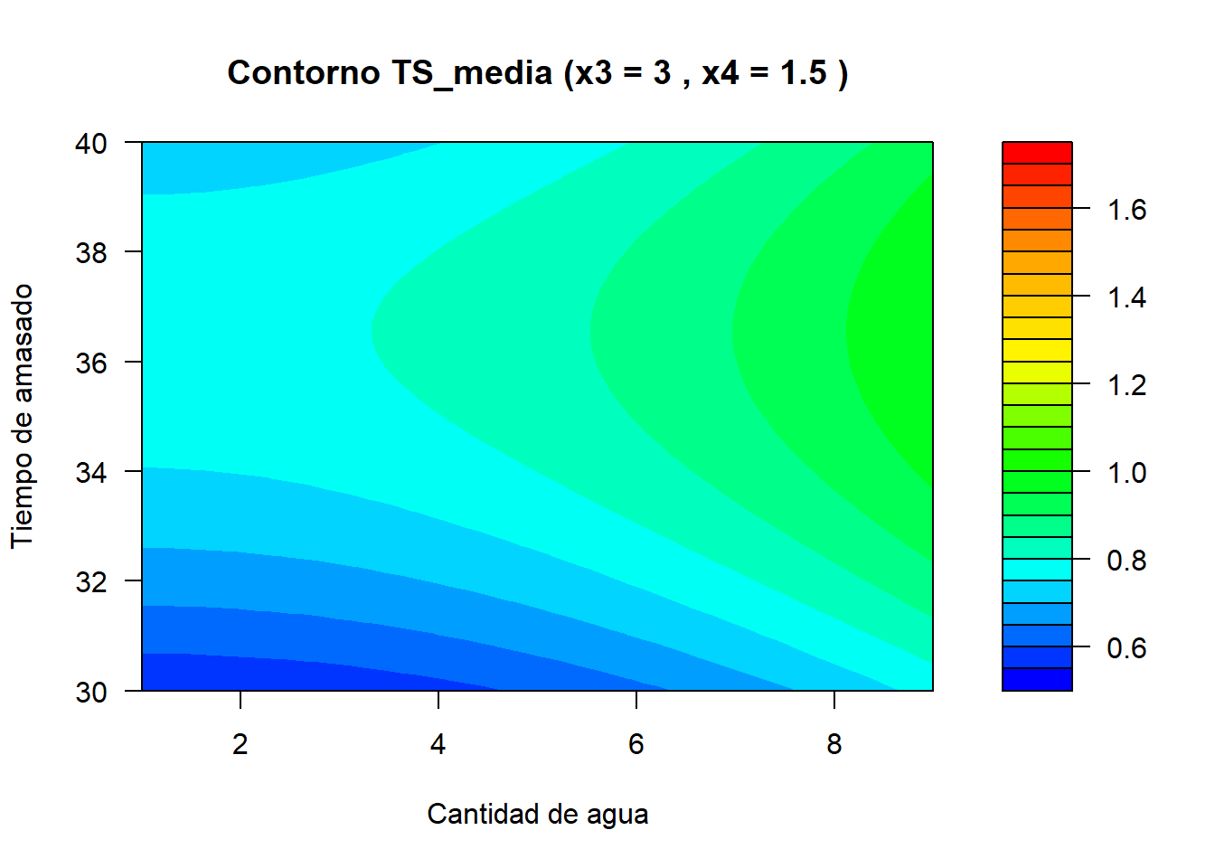
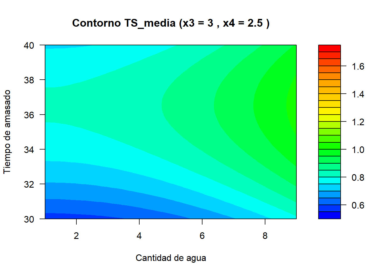
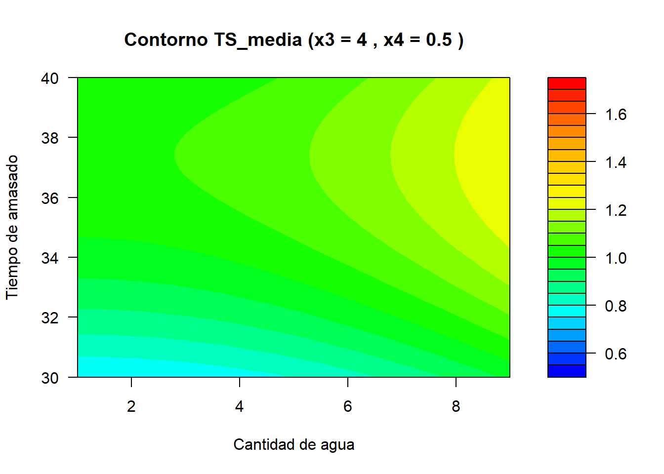
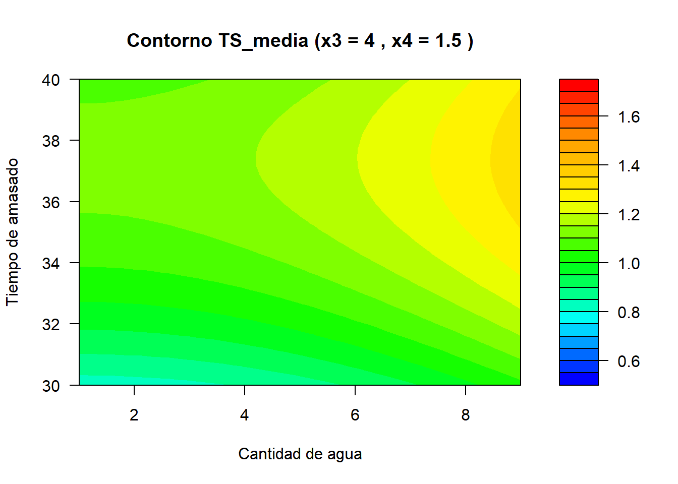
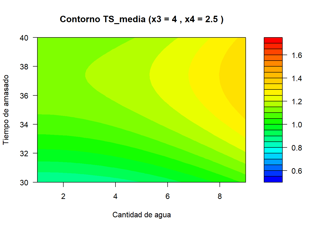
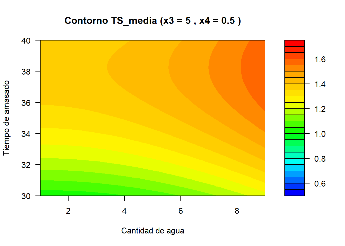
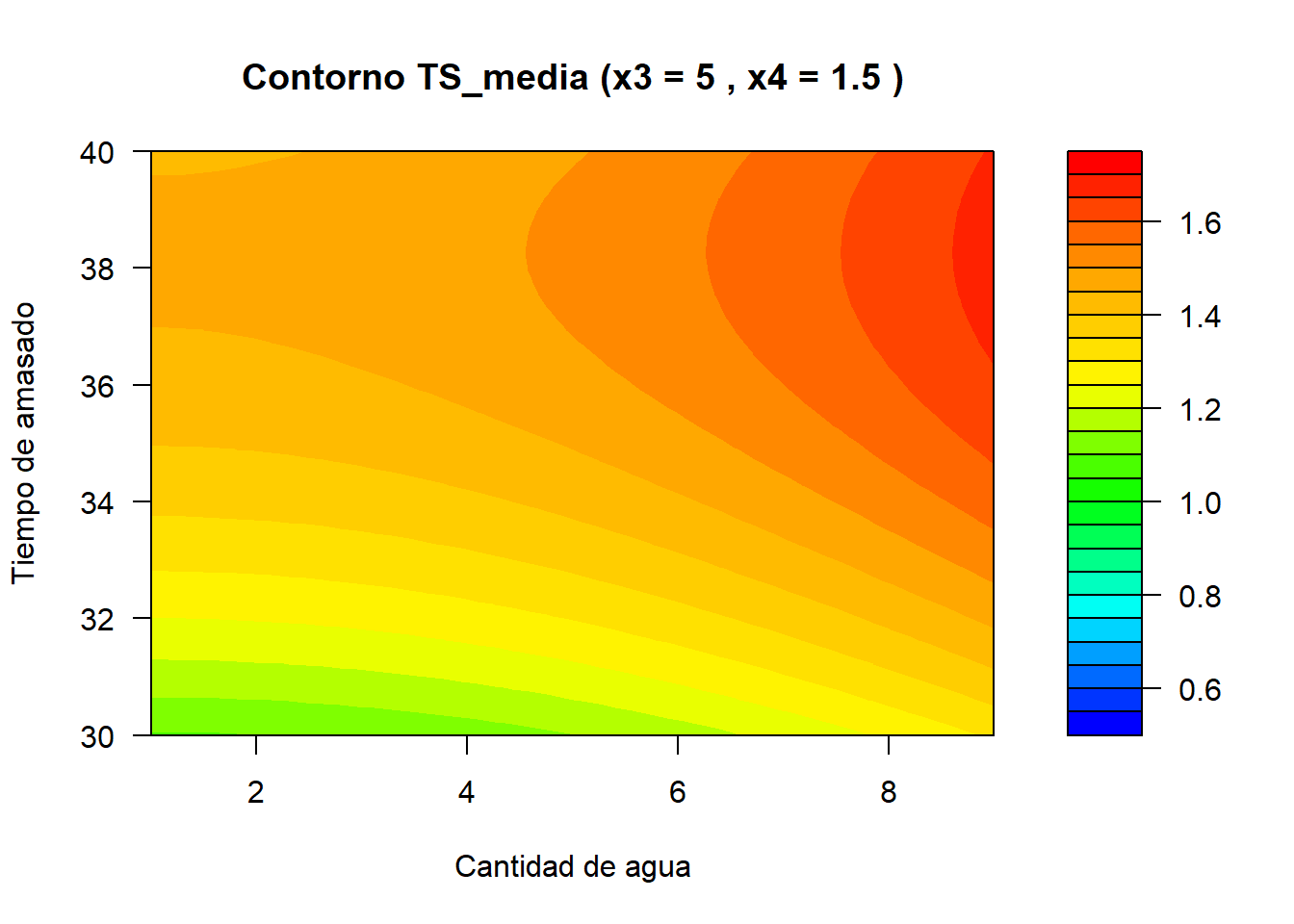
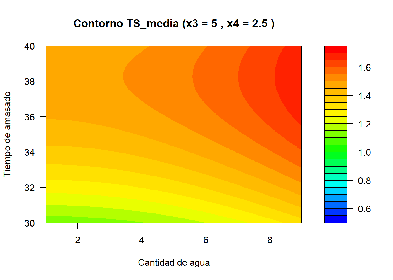
I(x1_nat^2) + I(x2_nat^2) + I(x4_nat^2), data = des)11 Gráficos de contorno
Código
# Valores para x3 y x4
#x3_vals <- c(-1, 0, 1)
#x4_vals <- c(-1, 0, 1)
x3_vals <- c(3, 4, 5)
x4_vals <- c(0.5, 1.5, 2.5)

# Secuencia de valores para x1 y x2
#x1_vals <- seq(-1, 1, length.out = 50)
#x2_vals <- seq(-1, 1, length.out = 50)
x1_vals <- seq(30, 40, length.out = 50)
x2_vals <- seq(1, 9, length.out = 50)

# Crear una ventana para 9 gráficos

for (x3_i in x3_vals) {
  for (x4_i in x4_vals) {

    # Crear grid para x1, x2 con x3_i y x4_i fijos
    grid <- expand.grid(x2_nat = x2_vals,
                        x1_nat = x1_vals,
                        x3_nat = x3_i,
                        x4_nat = x4_i)

    # Predecir TS_media
    grid$TS_hat <- predict(mod, newdata = grid)

    # Convertir a matriz para contour
    z <- matrix(grid$TS_hat, nrow = length(x2_vals), ncol = length(x1_vals), byrow = TRUE)

    # Graficar contorno con fondo coloreado
    filled.contour(x = x2_vals,
                   y = x1_vals,
                   z = z,
                   zlim = c(0.5, 1.75),
                   color.palette = colorRampPalette(c("blue", "cyan", "green", "yellow", "orange", "red")),
                   xlab = "Cantidad de agua",
                   ylab = "Tiempo de amasado",
                   main = paste("Contorno TS_media (x3 =", x3_i, ", x4 =", x4_i, ")"),
                   plot.axes = {
                     axis(1)
                     axis(2)})}}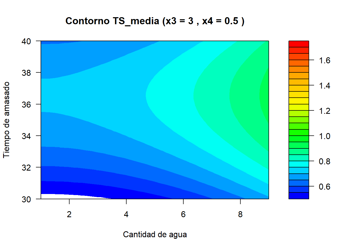
Hayashi, Yoshihiro. 2014. «Desarrollo de métodos QbD novedosos para comprender el proceso de fabricación de productos farmacéuticos». Tesis doctoral, Universidad de Ciencias Farmacéuticas de Hoshi.